

Demystifying Machine Learning
An Accessible Mathematical Exploration for Non-Mathematicians

Understanding the fundamental mathematical principles underlying machine learning is key for informed decision-making regarding its diverse applications among users, developers, and investors. Contrary to some perceptions, machine learning is not shrouded in mystery but rather grounded in systematic, logical mathematical functions that enable AI models to analyze data, detect patterns, and generate accurate predictions. With this post, I aim to provide a high-level overview of some foundational mathematical concepts that serve as the backbone of machine learning, framing the process as a sequence of structured, mathematical steps. While not delving into more advanced techniques, I believe these core ideas can establish baseline knowledge for appreciating the mathematical essence of even intricate AI systems. This understanding is particularly valuable in biomedicine, where distinguishing between the realistic capabilities of AI and overambitious assertions is imperative to avoid costly disappointments. A pragmatic comprehension of the types of problems AI can genuinely solve, and the mathematical means by which it does so, is key for stakeholders to make judicious choices about deploying these technologies safely, effectively, and responsibly.
Understanding Machine Learning Through Mathematical Functions
Machine learning can be easily understood by envisioning it as a series of mathematical functions. Under this framework, the learning algorithm can be represented by the function f(x), where x is the input and y is the output. The process of training an algorithm essentially involves applying the function f to the input x, yielding the output y. In mathematical language, we express this as:
This perspective provides an intuitive yet rigorous understanding of the basis for how machine learning algorithms operate at their core. The mathematical function f captures the essence of the computational process abstracted away from the technical details. “Learning,” in the context of machines, can be characterized as the optimization of mathematical functions through backpropagation and gradient descent discussed later in this post.
In practical applications, the input x might include patient data such as symptoms, medical histories, and diagnostic results, while the output y would be predictions or diagnoses, like identifying the presence of a disease, characterizing new patient subtypes, or forecasting patient outcomes. In essence, machine learning is a process of transforming input data into meaningful outputs through the development and refinement of algorithms using a variety of mathematical functions.
Functions can be linear or nonlinear, each representing different relationships between dependent (y) and independent (x) variables. A linear function is characterized by a constant rate of change, meaning that the relationship between the dependent and independent variables is proportional and represented by a straight line graphically (Figure-1). It can be expressed in the form:
where:
y is the outcome of interest (dependent variable)
m is the slope, representing the rate of change
x is the input (independent) variable
b is the y-intercept, denoting where the line crosses the y-axis when the input variable x = 0. This is also called bias in neural networks, allowing for the fine-tuning of predictions.
Nonlinear functions, on the other hand, are characterized by a variable rate of change, resulting in more complex relationships between dependent and independent variables. This variability manifests in their graphical representations, often as curves or intricate shapes rather than straight lines (Figure-1). A quintessential example of a non-linear function is the sigmoid function, represented as:
Where:
σ(x) is the sigmoid function itself. It's used to denote the output of the function, which ranges between 0 and 1.
x is the independent variable or input to the function (in a neural network, x could be a linear combination of input signals)
e is Euler's number, approximately equal to 2.71828
The sigmoid function is particularly notable for its S-shaped curve (sigmoid curve). As x approaches positive infinity, σ(x) approaches 1, and as x approaches negative infinity, σ(x) approaches 0.1
The key difference between linear and nonlinear functions is the consistency of their rate of change: Linear functions exhibit a constant rate of change, maintaining uniformity in how the output varies with respect to the input. In contrast, nonlinear functions show a variable rate of change, where the relationship between input and output is not uniform and can vary in different ranges of the input.
In reality, many biomedical relationships are complex and nonlinear. While linear models like Linear Regression are effective for situations where inputs (independent) and output (dependent) variables change proportionally, they often fall short of capturing the complexity of biological systems.

Nonlinear machine learning models are crucial for addressing the nuances of complex systems. These models include a wide range of techniques that include Artificial Neural Networks (ANNs), Bayesian Networks (BNs), Support Vector Machines (SVMs), and Decision Trees (DTs). Selecting the appropriate machine learning model for biomedical applications is a nuanced process, necessitating a careful balance between model complexity, interpretability, and accuracy.
Biomedical data often involve complex interactions among variables, requiring models that can capture these intricate relationships. While linear models like Linear Regression are transparent and straightforward, they can lack the sophistication to address the nonlinearity prevalent in many biological systems. On the other hand, more complex models, such as ANNs and SVMs, offer higher accuracy in capturing these nonlinear interactions but can be less interpretable. Ultimately, the decision must align with the specific requirements of the biomedical application, considering factors like the need for model transparency, the complexity of the data, and the criticality of prediction accuracy. Balancing these aspects ensures that the chosen model not only provides precise insights but also aligns with the ethical and practical demands of biomedical research and healthcare delivery.
Introducing Nonlinearity into Machine Learning Models
I will use neural networks as an example of how nonlinearity is incorporated into machine learning algorithms. These networks, structurally inspired by the human brain's network of neurons, are intricate systems comprised of interconnected nodes or neurons, each performing specific computational tasks.
Neural networks are arranged in layers: an input layer that receives data, several hidden layers that process the data, and an output layer that presents the final computation (Figure-2). The data input into the network undergoes a series of transformations as it propagates through these layers. The effectiveness of neural networks in handling complex, nonlinear tasks stems from their layered architecture and the operations performed within each layer.

The introduction of nonlinearity in neural networks is achieved through activation functions. An activation function, denoted as σ in mathematical terms, is applied to each neuron’s output in the desired layer where it can transform the linear input from the previous layer into a nonlinear output, enabling the network to learn and model complex relationships present in the data. This output sets the threshold for determining whether the neuron "fires" and sends a signal to the next layer. The final output is a product of complex patterns in nodal activation.
As mentioned previously, the operation of a neural network can be represented by the function y = f(x). The function f, which embodies the network’s computational process, is actually a composition of multiple functions representing the layers of the network. Each layer applies its own transformation (weights W and biases b), followed by the activation function σ. Mathematically, this can be expressed as follows for a single layer:
The role of this mathematical function in neural networks is pivotal. It encapsulates the entire process of data transformation, from the input layer through the hidden layers to the output layer. The function represents how the network processes input data (x), applies learned weights (or coefficients) and biases (W and b, respectively), and uses activation functions σ to produce the output y as a nonlinear or linear relationship between dependent and independent variables.
More sophisticated AI models essentially follow a similar logic. For example, the mathematical function for the attention mechanism of Transformers, which are behind the success of Large Language Models (LLMs) like ChatGPT, can be expressed as follows:
The above fancy-looking formula is basically y = f (x). Let’s break it down to illustrate:
Input (x). In the self-attention mechanism, the inputs are the matrices Q (queries), K (keys), and V (values). These matrices are derived from the input data (independent variables), which in the case of natural language processing (NLP) applications, is typically a sequence of word embeddings.
Function (f). The self-attention mechanism itself acts as the function f. This function involves:
Calculating a score (QK^T) that represents the alignment between different components of the input (such as different words in a sentence)
Scaling this score by dk to stabilize learning
Applying the softmax function to obtain a probability distribution (basically a type of activation function that also introduces nonlinearly)
Multiplying this distribution with the value matrix V
Output (y). The output of the self-attention mechanism is the result of the function applied to the input. This output is essentially a new representation of the input data, where each element now contains a weighted combination of its original features and the features of other elements in the sequence, as determined by their computed relevance or “attention.”
Features and Inputs
You've probably heard of phrases like "feature extraction" in machine learning. What exactly are these features? To understand this, it's helpful to first clarify the concepts of inputs and features in machine learning and statistical modeling.
Inputs and features are often mentioned interchangeably, as they both refer to the independent variables used by a model to predict or explain an outcome, which is the dependent variable. As mentioned previously, inputs are variables used to compute the output. In a general model context, inputs refer to any data provided to a model for processing or analysis. Often, features are derivatives or processed versions of simpler input variables, tailored to be more effective for machine learning. Features are often “extracted” from inputs through various processing techniques such as normalization, standardization, or more complex feature extraction methods. During model training, these features are fed into the algorithm as inputs, enabling it to learn patterns and make predictions (by calculating y in mathematical function language). In machine learning, we typically do feature extraction to transform the raw data into a set of numerical features to represent the data in a way that highlights the essential aspects.
Let’s represent the concept of features in machine learning function as a linear model for simplicity as an example. Consider a scenario where we are trying to predict a simple outcome based on multiple features. Let's say we have a dataset with features x_1,x_2,...,x_n and we want to predict a target variable y.
A basic linear model for this scenario can will look something like:
Where:
y is the target variable we want to predict
x_1, x_2,..., x_n are the features (inputs) of the dataset
b is the intercept of the model when inputs = 0
W_1, W_2, W_n are the weights (i.e., coefficients) for each feature, representing the weight or importance of each feature in the prediction2
The input layer in a neural network typically receives input features as input vectors. An input vector, usually denoted as X, is used to represent a collection of multiple inputs or features. In machine learning, each element of X could represent a different feature of a dataset. For example, in a dataset describing patients, X might include features like age, gender, vital signs, etc. Understanding the relationship and conceptual distinction between inputs, features, and vectors is essential for effective machine learning, as it impacts how well a model can learn and make accurate predictions.
Backpropagation and Gradient Descent
So how do neural networks actually evolve their structure during the learning process? This transformation occurs through the intricate mechanisms of backpropagation and gradient descent. Backpropagation, or "backward propagation of errors," involves several important steps. Initially, as we discussed, input data (x) moves forward through the layers of neurons, undergoing transformations via activation functions, weights, and biases, culminating in the network's prediction (y). The accuracy of this prediction is then assessed by comparing it to the actual target value by calculating the error or loss. This error measurement is crucial as it signifies the deviation of the network's prediction from the desired outcome. Basically, the error is the difference between y_predicted and y_true value.
Backpropagation begins with a backward pass to minimize this error by calculating the gradient of the error relative to each network weight (W) and bias (b), using the chain rule of calculus.3 This helps in determining the contribution of each W and b to the error. These gradients are then used to update the weights and biases, nudging them towards reducing the error. The learning rate plays a pivotal role in this process, controlling the magnitude of adjustments to W and b for balanced and effective learning.
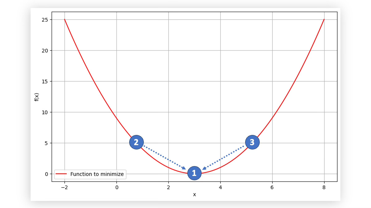
Gradient descent is a function optimization algorithm that iteratively adjusts the weights and biases to minimize the overall error or loss of the network. By taking steps proportional to the negative of the gradient, it ensures that the network parameters move towards reducing the error, leading to improved model performance (Figure-3).
Together, backpropagation and gradient descent make the neural network learning process both versatile and effective. This combination is applicable to a wide range of neural networks, including Convolutional Neural Networks (CNNs) and Recurrent Neural Networks (RNNs), and is vital in tasks from image recognition to language processing. Despite its computational demands, this duo proves efficient in handling the complexity of large neural networks, systematically enhancing model performance through iterative learning and optimization.
Let’s visualize the process using mathematical functions. Please feel fee to skip this part since it outlines the same concept described above although I encourage folks to follow along to see that mathematical functions are very rationally constructed and can be easy to understand.
Let’s consider a neural network as a function F in forward pass across the layers of neurons. Each neuron applies a specific transformation to its input (as we learned, the inputs are typically input vectors X but we’ll use x here for simplicity). These transformations are defined by weights W and biases b. For an input data x, the network computes its output y_predicted by successively applying these transformations. Mathematically, it can be represented as:
Where the function F encapsulates the complex operations (like activations and W, b operations) occurring inside the network.
The next step involves quantifying the error using a loss function L.4 When y_true value is the actual target value, the error E is:
Now let’s determine how much each weight and bias contributes to the error using backpropagation. This is done by computing the gradient of the error E with respect to each weight W and bias b in the network. Using the chain rule of calculus, we calculate:
These gradients indicate the direction and magnitude by which the weights and biases need to be adjusted to reduce the error.
Once the gradients are computed, we can start our gradient descent to adjust the weights and biases in the direction that would reduce the error. If α represents the learning rate, the weights and biases are updated as follows:
The learning rate controls how big a step we take in the direction of the gradient; too large can overshoot the minimum error (positioned at point 1 in Figure-3), too small can make the learning process very slow.
Supervised, Unsupervised, and Semi-Supervised Learning
Let’s continue with our mathematical function framework to explain supervised and unsupervised learning. In supervised learning, the process resembles fine-tuning the mathematical function f(x) based on known outputs (y), which are what we call labeled data for training. Imagine you have a set of inputs (input features or vectors) x and their corresponding known outputs y. The goal of training the model is to adjust f(x) so that it accurately predicts y for any given x. If the output of our function f(x) doesn't match the labeled data y, the algorithm iteratively minimizes this error by adjusting the function's parameters via backpropagation and gradient descent. Once trained through several runs (called epochs), the model learns the common characteristics of the training data.
In contrast, unsupervised learning does not involve labeled outputs. Instead, the algorithm tries to understand the structure of the data by identifying patterns, such as clusters or associations, without any predefined notion of what these patterns should be. It's like having a function f(x) that organizes data into meaningful structures without knowing in advance what these structures should look like. This approach is useful for discovering hidden patterns in data but does not directly predict or classify new data points based on learned labels, as there are none. The success of unsupervised learning heavily relies on the inherent characteristics of the data and the ability of the algorithm to capture and represent these characteristics effectively.
Semi-supervised learning combines elements of both supervised and unsupervised learning. This approach is typically utilized in scenarios where there is a limited amount of labeled data and a larger pool of unlabeled data. The fundamental concept of semi-supervised learning is to leverage the available labeled data to guide the learning process and then apply the insights gained to the unlabeled data to enhance the model's performance.
In practice, a model trained using semi-supervised learning begins by learning from a small set of labeled data. This initial learning phase provides the model with a foundational understanding. The model then uses this foundation to make predictions or identifications on the unlabeled data. These predictions are subsequently used to refine and improve the model's learning algorithm.
The primary advantage of semi-supervised learning lies in its efficiency, particularly regarding data utilization. It reduces the dependence on extensively labeled datasets, which can be costly and time-consuming to produce. This efficiency makes semi-supervised learning especially valuable in fields where labeled data is scarce or expensive to generate, such as medical diagnostics or complex language processing tasks.
Additionally, semi-supervised learning can potentially lead to more generalized models. By incorporating both labeled and unlabeled data in training, the models may develop a more holistic understanding of the data, potentially reducing the risk of overfitting. Overfitting occurs when a model is too closely tailored to the training data and fails to perform effectively on new, unseen data.
Inductive vs Deductive Reasoning
I conceptualize the complex processes in machine learning that lead to output prediction as computational reasoning. This mirrors the inductive and deductive reasoning we regularly apply in daily tasks, similarly adopted in computational reasoning frameworks within machine learning.
Inductive reasoning is a bottom-up process where conclusions are drawn from specific observations to broader generalizations and it is a staple in medical practice and research. For instance, physicians often start with specific observations, such as a patient's symptoms, medical history, and diagnostic results. They then draw broader generalizations or hypotheses based on these observations. For example, if a patient presents with symptoms like fever, cough, and chest pain, a physician may inductively hypothesize that the patient might have a respiratory infection. Inductive reasoning involves generalizing from specific data to make a probable diagnosis.5 Similarly, when we conduct a clinical trial and empirically observe that a specific therapy safely and effectively treats a disease in a statistically significant and clinically meaningful manner (FDA terminology alert!), we’re engaging in inductive reasoning to make broader conclusions about the therapy’s performance in the general population having the indicated disease.
In machine learning, this inductive approach is reflected in how algorithms learn from specific data instances, making generalizations that can be applied to new, unseen data. For example, a machine learning model might analyze numerous patient records containing clinical and diagnostic variables to learn patterns and generalize these to predict disease outcomes in future patients.
Inductive reasoning, whether performed by humans or machines, is probabilistic. That is, we can at best only estimate an outcome with a margin or error based on the information we receive/data we gather (the input variables). This applies to both conducting a clinical trial to estimate treatment safety and efficacy or a machine learning algorithm determining whether the input it receives is an image of a cat. In both cases, the reasoning is based on the analysis of available data to make a probable prediction.
Deductive reasoning, in contrast, operates from a top-down approach, starting with general principles or theories to form specific predictions or analyses. This method typically involves a hypothesis or a theoretical framework which is then tested through specific observations or experiments. In the context of clinical practice, physicians often employ deductive reasoning to make specific diagnoses using a general framework based on established clinical presentations and pathophysiology of disease. This mirrors the process in machine learning, where models apply general rules they have learned to make predictions on new, specific data. An example of this is a model using established genetic markers to predict diseases in individual patients, thereby testing and validating its foundational hypotheses.
The interplay of inductive and deductive reasoning supports critical decision-making processes in both scientific and clinical practices as well as in the field of computational reasoning. In machine learning, this dual approach allows for the development of biomedical models that not only learn from data but also rigorously test and validate the learnings, ensuring accuracy and reliability where outcomes can have significant implications for their intended use.
The Evolving Landscape of AI
By demystifying the core mathematical functions underpinning machine learning methods and elaborating on some of their practical applications, I hope I’ve been able to express the importance of having a core understanding of the mathematical concepts. This understanding goes beyond mere academic interest; it’s an important metric for informed decision-making in a rapidly evolving field that will transform many industries in the years to come. In biomedicine, where the stakes are high and the data increasingly complex, grasping the mathematical blueprints of machine learning can empower decision makers to differentiate between realistic AI capabilities and overreaching promises.
The exploration into the mathematical backbone of machine learning also highlights the significance of balancing simplicity and complexity in model selection; sometimes less can be more and often more is better. The key lies in choosing the right tool for the task at hand, considering the trade-offs between accuracy, interpretability, computational burden, and ethical implications.
As AI continues its integration into various facets of biomedicine, accompanied by ongoing discoveries in machine learning, its mathematical foundations will undoubtedly advance in parallel. Therefore, it's essential to have an understanding of the core mathematical principles to keep pace with the rapid evolution in the field. In a future post, I’ll delve into the basic mechanics of generative models and their potential applications in drug discovery and clinical research.
This property makes it useful for transforming values into a bounded range, often used in logistic regression and neural networks for classification tasks.
In machine learning, weights (i.e., coefficients) are vital as they help determine how significantly each feature (input variable) influences the prediction or outcome. We can think of them as the dials that the algorithm adjusts to understand and interpret data better. In a way, these weights are one of the key learning component of the algorithm: as the model is trained with data, it adjusts these weights to minimize errors in its predictions. The importance of each feature is quantified by its weight, which is crucial for both understanding and optimizing the model. For example, in a healthcare model predicting patient outcomes, a high coefficient for a feature like blood pressure would indicate its strong influence on the prediction.
Backpropagation optimizes neural networks by adjusting their weights (W) and biases (b) based on the error in predictions. The chain rule allows us to understand how small changes in W and b affect the overall error. It helps in calculating the gradient of the error with respect to each weight and bias, by breaking down the complex, multi-layered transformations of the neural network into simpler, manageable parts. Essentially, it tells us how to tweak the internal parameters of the network to minimize the prediction error, enabling the network to learn from data and improve its performance. Without the chain rule, the task of training deep neural networks, especially those with many layers, would be significantly more challenging and less efficient.
A loss function in machine learning measures how far a model's predictions deviate from the true values it aims to predict. For example, consider a model that predicts a patient's blood pressure based on inputs like age, weight, and medical history. The loss function would compare the model's predicted blood pressure to the patient's actual measured blood pressure. Loss functions guide the learning process by quantitatively measuring the model's performance on training data. Appropriate loss function design is key for optimizing a model to accurately predict continuous target variables like blood pressure. Loss functions provide a feedback signal to inform adjustments to model parameters.
After forming initial hypotheses through inductive reasoning, physicians apply deductive reasoning to refine and confirm their diagnoses. Deductive reasoning involves starting with a general principle or theory and applying it to specific cases. In the medical context, physicians use established medical knowledge and diagnostic criteria to deduce specific diagnoses. They may use deductive reasoning to rule out potential causes of symptoms and arrive at a final diagnosis based on deductive logic.